Change horizontal axis values. Select the axis values you want to format.
How To Edit Legend In Excel Excelchat
As a result we changed x axis values from Years to Stores.
. Formatting Excel Graphs Using VBA. Select the Format Axis option. On the Ribbon select the Chart Tools Format tab then click Format Selection.
Once open the Formatting Task pane remains available until you close it. In this go to the Number tab and expand it. Instead of trying to reformat the points using the legend to edit you need to click a single point of the scatter plot itself.
I can think of two ways to set up a legend like this. The Format Axis dialog box appears. Under Axis Options click Fixed for Base Unit and then in the Base Unit box click Days Months or Years.
In Excel 2003 it is necessary to transform the data to get the intended result. Similar to a legend we need to ensure the title exists before changing it to our liking. To do this manually using Excel.
Configure Text axis under the Axis Type option. You might try Excel Power Programming with VBA by John Walkenbach. Select Data on the chart to change axis values.
Open workbook in Excel. In Custom Axis Y 1 2 4 8 16 I showed axes with base 2 logarithmic scales in both Excel 2003 and 2007. After this use the Font dialog to change the size color and also add some text effects.
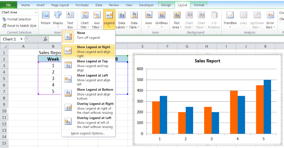
Also this legend includes the current value for each data series. When you click this command button Excel displays a menu of commands with each command corresponding to a location in which the chart legend can be placed. 2 In Excel 2007 and 2010s Format Axis dialog box click Number in left bar click to highlight the Percentage in the Category box and then.
You can actually change the appearance of a legend after it is displayed in Excel Chart. Right-click on the axis. In the Axis Options category under Axis Type make sure Date axis is selected.
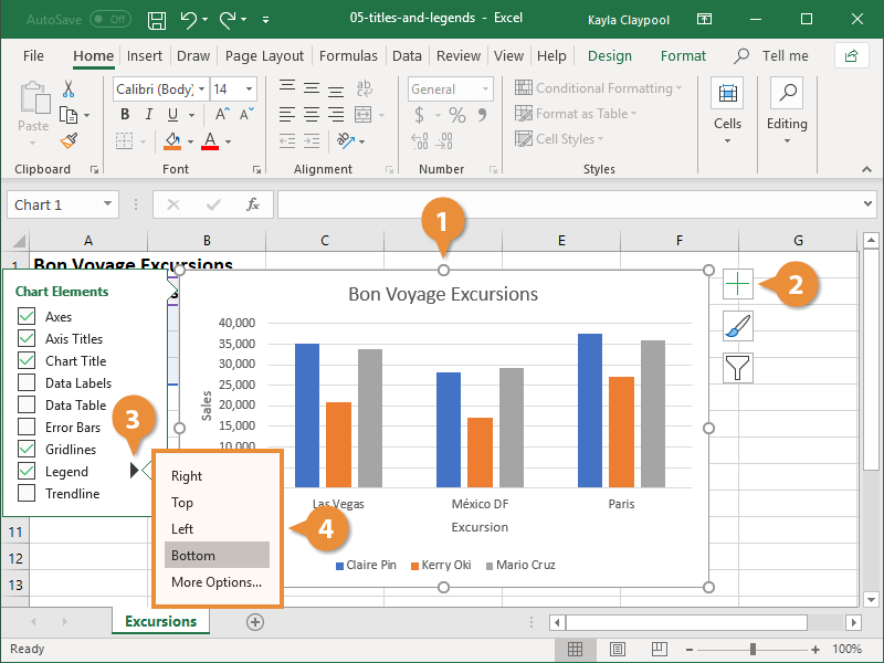
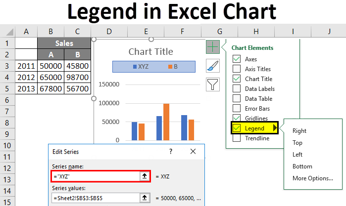
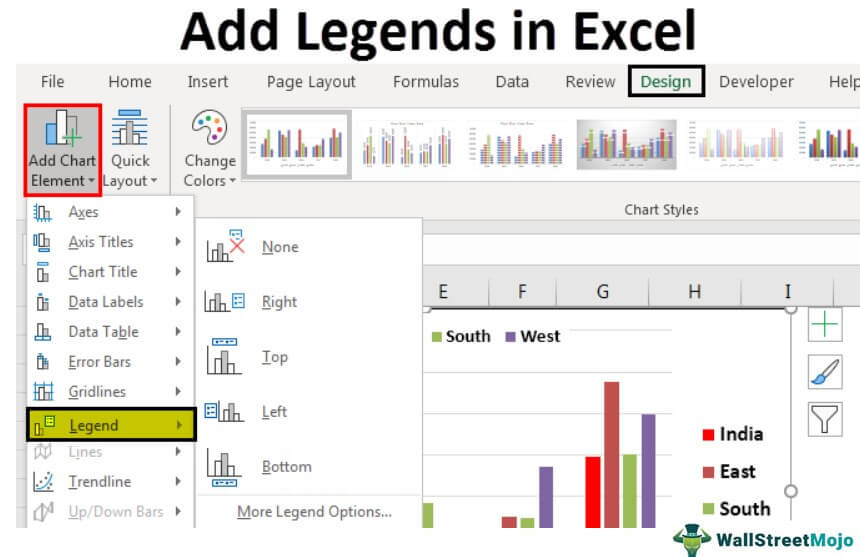
How to format an excel legend. A chart legend simply identifies the data series plotted in your chart. Click on the drop-down list of Add Chart Element Legends Legend Options.
You cannot have a date axis if the dates in your chart appear in the legend. Select the chart and go to Design. Because this chart shows random data the legends automatically adjust each time I recalculate my workbook.
Returns a Legend object that represents the legend for the chart. If you are using Excel 2007 2010 positioning of legend will not be available as shown in the above image. In Excel you can use the Add Chart Element Legend command on the Design tab to add or remove a legend to a pivot chart.
Select X axis chart. You may want to change the way that data is plotted in the chart so that. Change the Category to Percentage and on doing so the axis data points will now be shown in the form of percentages.
Select the new x-axis range. Click the x-axis or y-axis directly in the chart or click the Chart Elements button in the Current Selection group of the Format tab and then click Horizontal Category Axis for the x-axis. Select the Edit button and in the Axis label range select the range in the Store column.
You can add any other data you want of course. This example turns on the legend for Chart1 and then sets the legend font color to blue. By default the Decimal places will be of 2 digits in the percentage representation.
They are very approachable and still cover the material in a great deal of. In bar charts and charts that display a date axis the data table is not attached to the horizontal axis of the chart it is placed below the axis and aligned to the chart. In the above tool we need to change the legend positioning.
Y-Axis changes use xlValue and X-Axis changes use xlCategory. The issue is that the data set Im plotting uses dates on the x axis and Excel is intelligently filling in the gaps so if I have May 5 and May 7 in. The vertical axis is the xlValue axis and youll use Top and Height to figure how to center it.
The horizontal axis is the xlCategory axis and youll use Left and Width to figure how to center it. You can underline or even strikethrough. In this article.
In Excel 2007 the axis can be achieved with the untransformed data. Expression A variable that represents a Chart object. From there right click and choose the format data series option.
Under Design we have the Add Chart Element. One way would be to use a Camera object. Right-click then select Format where is the axis series legend title or area that was selected.
On a chart select an element. If you already display a legend in the chart you can clear the Show legend keys check box. 1 In Excel 2013s Format Axis pane expand the Number group on the Axis Options tab click the Category box and select Percentage from the drop down list and then in the Decimal Places box type 0.
To do this right-click on the legend and pick Font from the menu. If it is part of a series you should see the rest of the series selected as well.
Legends In Chart How To Add And Remove Legends In Excel Chart
How To Edit A Legend In Excel Customguide
Legends In Excel How To Add Legends In Excel Chart


0 Comments